First steps in Python

Dr.Jit offers both Python and C++ interfaces. The majority of this documentation covers the Python interface. For differences that are specific to C++, see the separate section on this.

Installing Dr.Jit

The easiest way to obtain Dr.Jit is using binary wheels, which we provide for officially supported Python versions and the most common platforms (Linux x86_64, Windows x86_64, macOS arm64/x86_64). To install Dr.Jit in this way, run

$ pip install drjit

The remainder of this section walks through a simple example that makes use of various system features. In particular, we will render an image of a bumpy sphere expressed as a signed distance function using just-in-time compilation, random number generation, GPU texturing, loop recording, and automatic differentiation. You can follow the example by copy-pasting code to a python file or a Juypter lab instance (recommended).

Importing Dr.Jit

Most Dr.Jit functionality resides in the drjit namespace that we typically associate with the dr alias for convenience.

import drjit as dr

Besides this, we must also choose a set of array types from a specific computation backend. Several choices are available:

• drjit.cuda provides data types for GPU-accelerated parallel computing using CUDA.

• drjit.llvm provides data types for CPU-accelerated parallel computing using the LLVM compiler infrastructure.

• drjit.scalar provides simple data types for serial/scalar computation.

Further backends (e.g. Apple Metal, Intel Xe) are planned in the future. The CUDA and LLVM backends also provide specialized aliases for derivative tracking using automatic differentiation (drjit.cuda.ad and drjit.llvm.ad). We will discuss them later as part of this tutorial.

We begin by importing various components that will be used in the tutorial:

from drjit.cuda import Float, UInt32, Array3f, Array2f, TensorXf, Texture3f, PCG32, Loop

LLVM backend

If you don’t have a CUDA-compatible GPU, change drjit.cuda to drjit.llvm in the above import statement. In that case, note that LLVM 8 or newer must be installed on the system, which may require additional steps depending on your platform:

• Linux: apt-get install llvm (or an equivalent command for your distribution.)

• macOS: brew install llvm using Homebrew.

• Windows: run one of the official installers (many files can be downloaded from this page, look for ones with the pattern LLVM-<version>-win64.exe). It is important that you let the installer adjust the %PATH% variable so that the file LLVM-C.dll can be found by Dr.Jit.

With that out of the way, let’s get back to the example.

Signed distance functions and sphere tracing

A signed distance function is a function that specifies the distance to the nearest surface. It provides a convenient and general way of encoding 3D shape information. We will initially start with a simple SDF of a sphere with radius 1 that is centered around the origin:

def sdf(p: Array3f) -> Float:
    return dr.norm(p) - 1

The function takes 3D points and returns the associated distance value. The type annotations are provided for clarity and can be omitted in practice. We can use an interactive Python prompt to pass an Array3f instance representing a 3D point into the function and observe the calculated distance.

>>> sdf(Array3f(1, 2, 3))
[2.7416574954986572]

The CUDA and LLVM backends of Dr.Jit vectorize and parallelize computation. This means that types like Float and Array3f typically hold many values at once that are used to perform simultaneous evaluations of a function. For example, we can compute the SDF at positions \((0, 0, 0)\) and \((1, 2, 3)\) in one combined step.

>>> sdf(Array3f([0, 1], [0, 2], [0, 3]))
[-1.0, 2.7416574954986572]

To visualize the surface encoded by the SDF, we will use an algorithm called sphere tracing. Given a ray with an origin \(\textbf{o}\) and direction \(\textbf{d}\), sphere tracing evaluates \(\mathrm{sdf}(\textbf{o})\) to find the distance of the nearest surface. The line segment connecting \(\textbf{o}\) and \(\mathbf{o} + \mathbf{d}\cdot\mathrm{sdf}(\textbf{o})\) is free of surfaces by construction, and the algorithm thus skips to the end of this interval. Further repetition of this recipe causes the method to either approach the nearest surface intersection \(\textbf{p}\) (visualized below) or escape to infinity.

The following sphere tracer runs for 10 fixed iteration and lacks various common optimizations for simplicity. The function fma() performs a fused multiply-add, i.e., it evaluates fma(a, b, c) = a*b + c with reduced rounding error and better performance.

def trace(o: Array3f, d: Array3f) -> Array3f:
    for i in range(10):
        o = dr.fma(d, sdf(o), o)
    return o

So far, so good. Now suppose p = trace(o, d) finds an intersection p. To use this information to create an image, we must shade it (i.e., assign an intensity value).

Many different shading models exist; a simple approach is to compute inner product of the surface normal and the direction \(\mathbf{l}\) towards a light source. Intuitively, the surface becomes brighter as it more directly faces the light source. In the case of a signed distance function, the surface normal at \(\mathbf{p}\) is given by the gradient vector \(\nabla \mathrm{sdf}(\mathbf{p})\) so that this shading model entails computing

\[\mathrm{max}\{0, \nabla \mathrm{sdf}(\mathbf{p}) \cdot \mathbf{l}\}\]

The gradient can be estimated using central finite differences with step size eps=1e-3, which yields the following rudimentary shading routine (we will improve upon it shortly).

def shade(p: Array3f, l: Array3f, eps: float = 1e-3) -> Float:
    n = Array3f(
        sdf(p + [eps, 0, 0]) - sdf(p - [eps, 0, 0]),
        sdf(p + [0, eps, 0]) - sdf(p - [0, eps, 0]),
        sdf(p + [0, 0, eps]) - sdf(p - [0, 0, eps])
    ) / (2 * eps)
    return dr.maximum(0, dr.dot(n, l))

To create an image, we must generate a set of rays that will be processed by these functions. We begin by creating a Float array with 1000 linearly spaced elements covering the interval \([-1, 1]\) and then expand this into a set of \(1000\times 1000\) \(x\) and \(y\) grid coordinates. The linspace() and meshgrid() functions resemble their eponymous counterparts in array programming libraries like NumPy.

x = dr.linspace(Float, -1, 1, 1000)
x, y = dr.meshgrid(x, x)

This is a good point for a small digression to explain a major difference to tools like NumPy.

Tracing and delayed evaluation

In most array programming frameworks, the previous two commands would have created arrays representing actual data (grid coordinates in this example).

Dr.Jit uses a different approach termed tracing to delay the evaluation of computation. In particular, no arithmetic took place during the two preceding steps: instead, Dr.Jit recorded a graph representing the sequence of steps that are needed to eventually compute x and y (which are represented by the bottom two nodes in the visualization below).

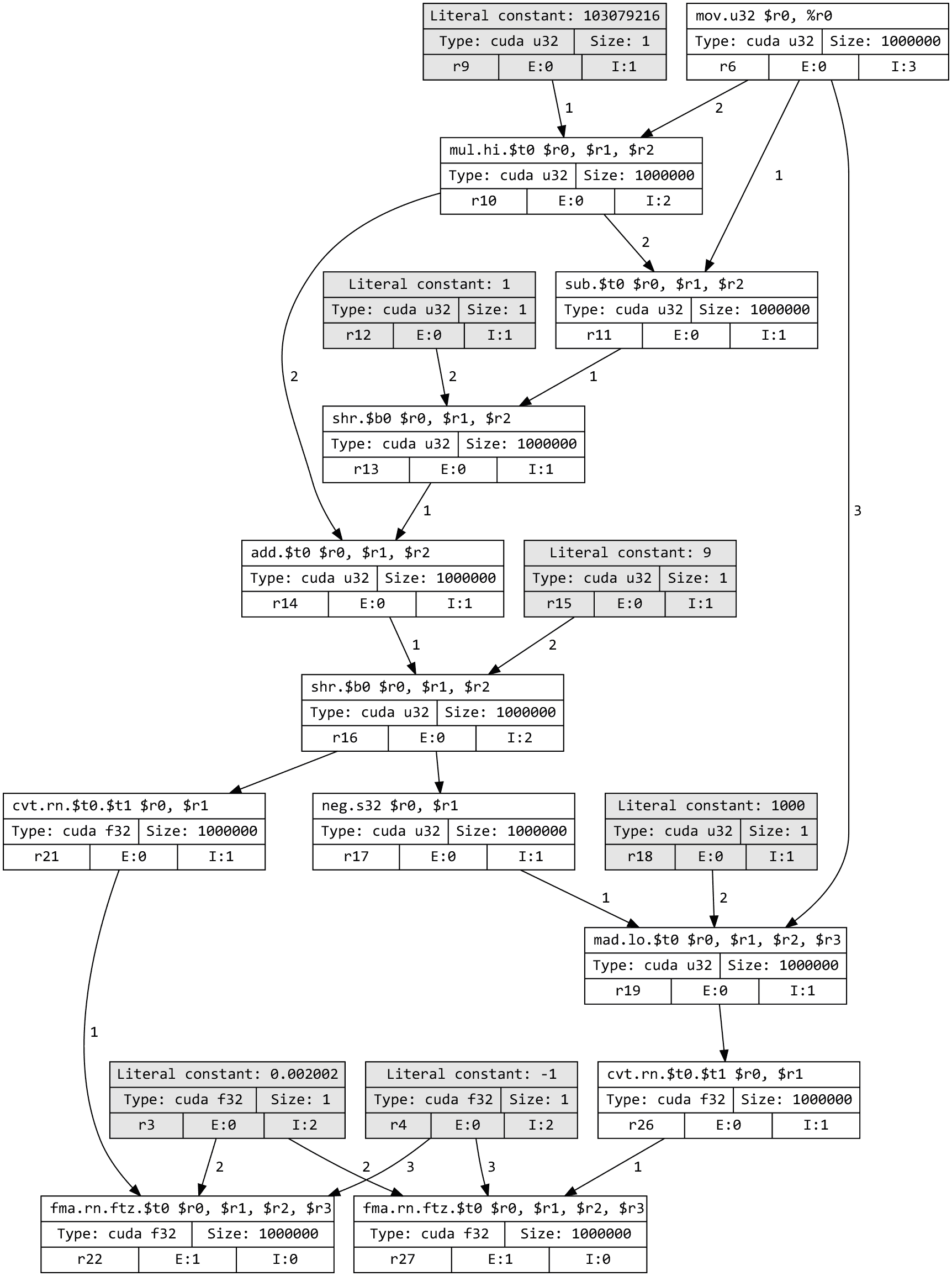
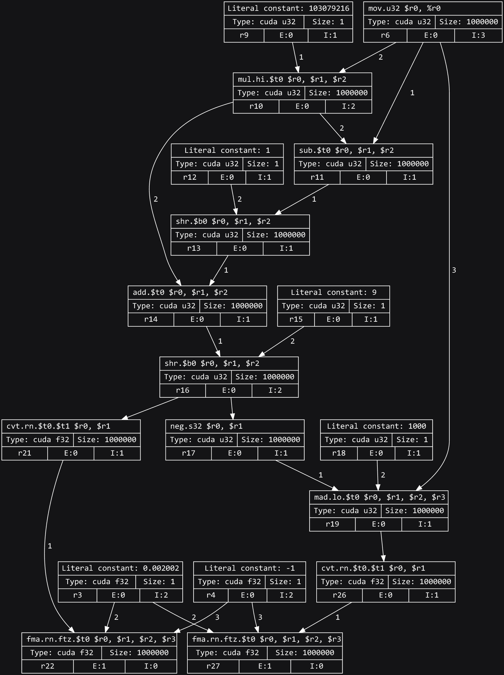
Note

To view a computation graph like this on your own machine, you must install GraphViz on your system along with the graphviz Python package. Following this, you can run dr.graphviz().view().

It is clear that the evaluation can not be postponed arbitrarily: we will eventually want to look at the generated image. At this point, Dr.Jit will take all recorded steps, compile them into an optimized kernel, and run it on the GPU or CPU. This all happens transparently behind the scenes.

What are the benefits of doing things in this way? Merging multiple steps of a computation into a kernel (often called fusion) means that these steps can exchange information using fast register memory. This allows them to spend more time on the actual computation as opposed to reading and writing main memory (which is slow). Tracing also opens up other optimization opportunities explained in the paper and video explaining the system’s design. Dr.Jit can trace enormously large programs without interruption and use the graph representation to simplify them.

Example, continued

We will now use the previously computed grid points to define a virtual camera plane with pixel positions \((x, y, 1)\) relative to a pinhole at \((0, 0, -2)\) and simultaneously perform sphere tracing along every associated ray.

p = trace(o=Array3f(0, 0, -2),
          d=dr.normalize(Array3f(x, y, 1)))

Next, we can shade the intersected points for light arriving from direction \((0, -1, -1)\). Note the masked assignment at the bottom, which disables shading for rays that did not intersect anything.

sh = shade(p, l=Array3f(0, -1, -1))
sh[sdf(p) > .1] = 0

We multiply and offset the shaded value with an ambient and highlight color. The resulting variable img associates an RGB color value with every pixel.

img = Array3f(.1, .1, .2) + Array3f(.4, .4, .2) * sh

If you are used to array programming frameworks like NumPy/PyTorch, it may be tempting to think of img as a tensor that points to a 3xN or Nx3-shaped block of memory (where N is the pixel count).

Dr.Jit instead traces computation for delayed evaluation, which means that no actual computation has occurred so far. The 3D array img (type drjit.cuda.Array3f) consists of 3 components (img.x, img.y, and img.z) of type drjit.cuda.Float, of which each represents an intermediate variable within a steadily growing program of the following high-level structure.

# For illustration only, not part of the running example

for i in range(1000000): # (in parallel)
    # .. earlier steps ..
    img_x = .1 + .4 * sh
    img_y = .1 + .4 * sh
    img_z = .2 + .2 * sh

This program performs a parallel loop over \(1000\times1000\) pixels. Subsequent Dr.Jit operations will simply add further steps to this program. For example, we can invoke ravel() to flatten the 3D array into a drjit.cuda.Float array.

img_flat = dr.ravel(img)

Conceptually, this adds three more lines to the program

# For illustration only, not part of the running example

for i in range(1000000): # (in parallel)
    # .. earlier steps ..
    img_flat[i*3 + 0] = img_x
    img_flat[i*3 + 1] = img_y
    img_flat[i*3 + 2] = img_z

This is essentially metaprogramming: running the program generates another program that will run at some later point and perform the actual computation. This all happens automatically and is key to the efficiency of Dr.Jit.

Dr.Jit also supports arbitrarily sized tensors of various types (for example, drjit.cuda.TensorXf for a CUDA float32 tensor). Tensors are useful for data exchange with other array programming frameworks. For example, we can reshape the flat image buffer into a \(1000\times 1000\times 3\) image tensor and then visualize it using matplotlib.

img_t = TensorXf(img_flat, shape=(1000, 1000, 3))

import matplotlib.pyplot as plt
plt.imshow(img_t)
plt.show()

Warning

Despite the presence of a tensor type, Dr.Jit is not a tensor/array programming library. Heavy use of tensor operations like slice-based indexing may lead to poor performance, since they impede Dr.Jit’s ability to fuse many operations into large kernels.

Programs should be mainly written in terms of 1D arrays (drjit.cuda.Float, drjit.cuda.UInt32, drjit.cuda.Int64, etc.) and fixed-size combinations. For example, drjit.cuda.Matrix4f wraps \(4\times 4=16\) drjit.cuda.Float instances, each of which represents a variable in the program.

The line plt.imshow(img_t) will access the image contents, and it is at this point that the traced program runs on the GPU, producing the following output:

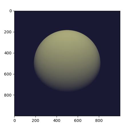
Complete example code up to this point.

import drjit as dr
from drjit.cuda import Float, UInt32, Array3f, Array2f, TensorXf, Texture3f, PCG32, Loop

def sdf(p: Array3f) -> Float:
    return dr.norm(p) - 1

def trace(o: Array3f, d: Array3f) -> Array3f:
    for i in range(10):
        o = dr.fma(d, sdf(o), o)
    return o

def shade(p: Array3f, l: Array3f, eps: float = 1e-3) -> Float:
    n = Array3f(
        sdf(p + [eps, 0, 0]) - sdf(p - [eps, 0, 0]),
        sdf(p + [0, eps, 0]) - sdf(p - [0, eps, 0]),
        sdf(p + [0, 0, eps]) - sdf(p - [0, 0, eps])
    ) / (2 * eps)
    return dr.maximum(0, dr.dot(n, l))

x = dr.linspace(Float, -1, 1, 1000)
x, y = dr.meshgrid(x, x)

p = trace(o=Array3f(0, 0, -2),
          d=dr.normalize(Array3f(x, y, 1)))

sh = shade(p, l=Array3f(0, -1, -1))
sh[sdf(p) > .1] = 0

img = Array3f(.1, .1, .2) + Array3f(.4, .4, .2) * sh
img_flat = dr.ravel(img)

img_t = TensorXf(img_flat, shape=(1000, 1000, 3))

import matplotlib.pyplot as plt
plt.imshow(img_t)
plt.show()

Textures, random number generation

This previous example was a little bland—let’s make it more interesting! We will deform the sphere by perturbing the implicitly defined surface with a noise function.

Dr.Jit was originally designed for Monte Carlo methods that heavily rely on random sampling, and it ships with Melissa O’Neill’s PCG32 pseudorandom number generator to help with such applications.

Here, we use PCG32 to generate a relatively small set of uniformly distributed variates covering the interval \([0, 1]\).

noise = PCG32(size=16*16*16).next_float32()

We can then create a noise texture from these uniform variates. The command below allocates a 3D texture with a resolution of \(16\times16\times 16\) and \(1\) color channel.

noise_tex = Texture3f(TensorXf(noise, shape=(16, 16, 16, 1)))

We finally replace the sdf() function with a modified version that evaluates the texture with an offset and scaled value of p to slightly perturb the level set. This uses the GPU texture units on the CUDA backend and a software-interpolated lookup in the LLVM backend.

def sdf(p: Array3f) -> Float:
    sdf_value = dr.norm(p) - 1
    sdf_value += noise_tex.eval(dr.fma(p, 0.5,  0.5))[0] * 0.1
    return sdf_value

Let us also add the following line at the beginning of the program, which causes Dr.Jit to emit a brief message whenever it compiles and runs a kernel.

dr.set_log_level(dr.LogLevel.Info)

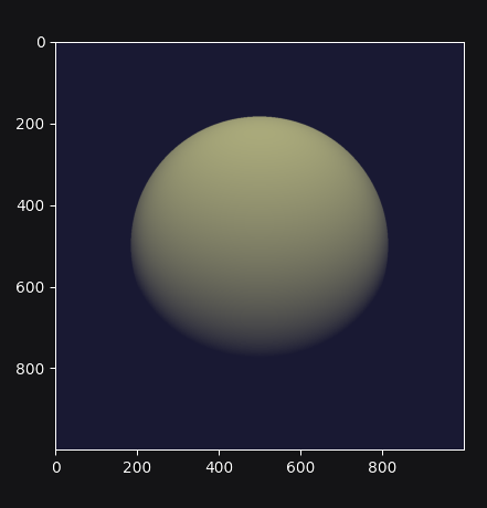
Re-running the program produces the following output:

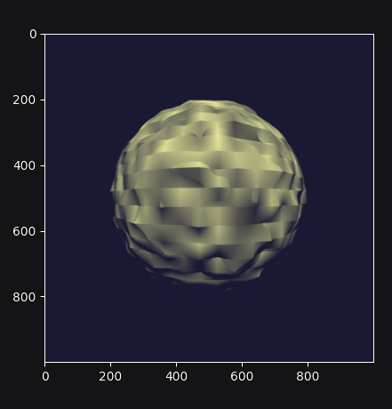
Why does it look so faceted? The texture uses trilinear interpolation, and the surface normal is given by the derivative of the interpolant (meaning that it will be piecewise constant). Dr.Jit also provides higher-order tricubic interpolation that internally reduces to eight hardware-accelerated texture lookups. We can use it to redefined sdf() once more:

def sdf(p: Array3f) -> Float:
    sdf_value = dr.norm(p) - 1
    sdf_value += noise_tex.eval_cubic(dr.fma(p, 0.5,  0.5))[0] * 0.1
    return sdf_value

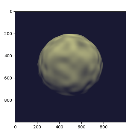
With this implementation, we obtain a smooth bumpy sphere.

Complete example code up to this point.

import drjit as dr
from drjit.cuda import Float, UInt32, Array3f, Array2f, TensorXf, Texture3f, PCG32, Loop

dr.set_log_level(dr.LogLevel.Info)

noise = PCG32(size=16*16*16).next_float32()
noise_tex = Texture3f(TensorXf(noise, shape=(16, 16, 16, 1)))

def sdf(p: Array3f) -> Float:
    sdf_value = dr.norm(p) - 1
    sdf_value += noise_tex.eval_cubic(dr.fma(p, 0.5,  0.5))[0] * 0.1
    return sdf_value

def trace(o: Array3f, d: Array3f) -> Array3f:
    for i in range(10):
        o = dr.fma(d, sdf(o), o)
    return o

def shade(p: Array3f, l: Array3f, eps: float = 1e-3) -> Float:
    n = Array3f(
        sdf(p + [eps, 0, 0]) - sdf(p - [eps, 0, 0]),
        sdf(p + [0, eps, 0]) - sdf(p - [0, eps, 0]),
        sdf(p + [0, 0, eps]) - sdf(p - [0, 0, eps])
    ) / (2 * eps)
    return dr.maximum(0, dr.dot(n, l))

x = dr.linspace(Float, -1, 1, 1000)
x, y = dr.meshgrid(x, x)

p = trace(o=Array3f(0, 0, -2),
          d=dr.normalize(Array3f(x, y, 1)))

sh = shade(p, l=Array3f(0, -1, -1))
sh[sdf(p) > .1] = 0

img = Array3f(.1, .1, .2) + Array3f(.4, .4, .2) * sh
img_flat = dr.ravel(img)

img_t = TensorXf(img_flat, shape=(1000, 1000, 3))

import matplotlib.pyplot as plt
plt.imshow(img_t)
plt.show()

Kernel launches, caching

Besides generating an image, the last experiment also produced several log messages enabled by the call to dr.set_log_level().

jit_eval(): launching 1 kernel.
  -> launching 17509add1324abde (n=4096, in=0, out=1, ops=41, jit=15.073 us):
     cache miss, build: 576.932 us, 3.375 KiB.
jit_eval(): done.
jit_eval(): launching 1 kernel.
  -> launching 87908afce75f85b5 (n=1000000, in=5, out=0, se=3, ops=2114, jit=330.965 us):
     cache miss, build: 1.17021 ms, 30.38 KiB.
jit_eval(): done.

Several things are noteworthy here:

• Dr.Jit launched two kernels: the first one to compute the noise texture with n=4096 texels, followed by the main rendering step that computed n=1000000 image pixels.

• The second kernel is big and contains over two thousand operations (ops=2114).

• It generated those kernels for the first time (cache miss) and so had to perform a somewhat expensive compilation step to generate machine code.

  If you re-run the example a second time, this part of the message will change to cache hit, and the compilation is skipped. Dr.Jit stores cached kernels on disk in the ~/.drjit directory on Linux/macOS, and in ~/AppData/Local/Temp/drjit on Windows. Dr.Jit was originally designed to accelerate gradient-based optimization; caching is particularly useful in this context, since the expensive compilation step will only run once during the first gradient step.

• If you are using the LLVM backend, the kernel will be even larger..

  jit_eval(): launching 1 kernel.
    -> launching 6e8cadb52477dd91 (n=1000000, in=5, out=0, se=3, ops=7560, jit=2.92385 ms):
       cache miss, build: 2.411 s, 78.25 KiB.
  jit_eval(): done.
  

  The CPU does not have hardware texturing instructions and must emulate them, which causes this size increase to over 7K instructions. While tracing is fast (2.9 milliseconds), the one-time compilation step now takes almost 2.5 seconds!

What leads to these large kernels? Not only does the bumpy sphere SDF generate more code: Dr.Jit’s computation graph also contains it a whopping 17 times: 10 times for sphere tracing steps, 6 times for finite differences-based normal computation, and one final time for the masked assignment that disables pixels without valid intersections. This doesn’t seem like a good way of using the system—let’s improve the example!

Recorded loops

A first inefficiency is that a normal Python for loop will unroll the loop many times, producing an unnecessarily large trace that is expensive to compile. It is also inflexible: there is no easy way to to stop the sphere tracing iteration early when it is sufficiently close to the surface.

Dr.Jit provides a recorded loop primitive to address these and related limitations. To use it, replace the earlier sphere tracing implementation

# Old version
def trace(o: Array3f, d: Array3f) -> Array3f:
    for i in range(10):
        o = dr.fma(d, sdf(o), o)
    return o

by the following improved version:

# Improved version
def trace(o: Array3f, d: Array3f) -> Array3f:
    i = UInt32(0)
    loop = Loop("Sphere tracing", lambda: (o, i))
    while loop(i < 10):
        o = dr.fma(d, sdf(o), o)
        i += 1
    return o

Expressed in this form, Dr.Jit will only trace the body once and make note of the fact that it must loop on the device while the condition i < 10 holds. The condition is itself a Dr.Jit array, and elements can therefore run the loop for different numbers of iterations.

For this all to work correctly, Dr.Jit needs to know what variables are modified by the loop body. The lambda: (o, i) parameter serves this role and allows the system to detect when variables are changed or entirely overwritten. The label "Sphere tracing" will be added to generated PTX/LLVM code and can be helpful when looking at kernels of programs containing many loops. This simple change reduces the operation count to half.

Automatic differentiation

Next, we can examine the shade() method that evaluated the SDF 6 times to compute an approximate derivative, which was a source of inefficiency:

# Old version
def shade(p: Array3f, l: Array3f, eps: float = 1e-3) -> Float:
    n = Array3f(
        sdf(p + [eps, 0, 0]) - sdf(p - [eps, 0, 0]),
        sdf(p + [0, eps, 0]) - sdf(p - [0, eps, 0]),
        sdf(p + [0, 0, eps]) - sdf(p - [0, 0, eps])
    ) / (2 * eps)
    return dr.maximum(0, dr.dot(n, l))

Dr.Jit includes an automatic differentiation layer to analytically differentiate expressions, producing code that is more efficient and more accurate. To use the AD layer, simple append .ad to the import directive at the top of the program. For example for the CUDA backend, you would write:

from drjit.cuda.ad import Float, UInt32, Array3f, Array2f, TensorXf, Texture3f, PCG32, Loop

There is essentially no extra cost for using types from the .ad namespace when gradient tracking isn’t explicitly enabled for a variable, so you can simply use them everywhere by default.

The AD version of shade() invokes drjit.enable_grad() to track the differential dependence of subsequent variables on the position p. It subsequently evaluates the SDF just once, which records the structure of the computation into a graph representation. The next two lines set an input gradient at p and propagate the derivative to the output value, which results in the desired directional derivative \(\nabla \mathrm{sdf}(\mathbf{p}) \cdot \mathbf{l}\).

# Improved version
def shade(p: Array3f, l: Array3f) -> Float:
    dr.enable_grad(p)
    value = sdf(p)
    dr.set_grad(p, l)
    dr.forward_to(value)
    return dr.maximum(0, dr.grad(value))

The dr.forward_to() call materializes the AD-based derivatives into ordinary computation that is traced along with the rest of the program.

This reduces the operation count by another factor of 2, and compilation time is now consistently between 30-90 milliseconds across backends.

Complete example code including optimizations

import drjit as dr
from drjit.cuda.ad import Float, UInt32, Array3f, Array2f, TensorXf, Texture3f, PCG32, Loop

dr.set_log_level(dr.LogLevel.Info)

noise = PCG32(size=16*16*16).next_float32()
noise_tex = Texture3f(TensorXf(noise, shape=(16, 16, 16, 1)))

def sdf(p: Array3f) -> Float:
    sdf_value = dr.norm(p) - 1
    sdf_value += noise_tex.eval_cubic(dr.fma(p, 0.5,  0.5))[0] * 0.1
    return sdf_value

def trace(o: Array3f, d: Array3f) -> Array3f:
    i = UInt32(0)
    loop = Loop("Sphere tracing", lambda: (o, i))
    while loop(i < 10):
        o = dr.fma(d, sdf(o), o)
        i += 1
    return o

def shade(p: Array3f, l: Array3f, eps: float = 1e-3) -> Float:
    dr.enable_grad(p)
    value = sdf(p);
    dr.set_grad(p, l)
    dr.forward_to(value)
    return dr.maximum(0, dr.grad(value))

x = dr.linspace(Float, -1, 1, 1000)
x, y = dr.meshgrid(x, x)

p = trace(o=Array3f(0, 0, -2),
          d=dr.normalize(Array3f(x, y, 1)))

sh = shade(p, l=Array3f(0, -1, -1))
sh[sdf(p) > .1] = 0

img = Array3f(.1, .1, .2) + Array3f(.4, .4, .2) * sh
img_flat = dr.ravel(img)

img_t = TensorXf(img_flat, shape=(1000, 1000, 3))

import matplotlib.pyplot as plt
plt.imshow(img_t)
plt.show()

Dr.Jit can propagate derivatives in forward mode (shown here) and reverse mode, which is useful for gradient-based optimization of programs with many inputs.

This concludes the running example. For those interested in the nitty-gritty details and quality of the generated code, we include an example of the PTX output produced by Dr.Jit below.

PTX intermediate representation produced by this example

.version 6.0
.target sm_60
.address_size 64

.entry drjit_b6460a9f61ed83ee22ab62b4db19ee5b(.param .align 8 .b8 params[48]) {
    .reg.b8   %b <398>; .reg.b16 %w<398>; .reg.b32 %r<398>;
    .reg.b64  %rd<398>; .reg.f32 %f<398>; .reg.f64 %d<398>;
    .reg.pred %p <398>;

    mov.u32 %r0, %ctaid.x;
    mov.u32 %r1, %ntid.x;
    mov.u32 %r2, %tid.x;
    mad.lo.u32 %r0, %r0, %r1, %r2;
    ld.param.u32 %r2, [params];
    setp.ge.u32 %p0, %r0, %r2;
    @%p0 bra done;

    mov.u32 %r3, %nctaid.x;
    mul.lo.u32 %r1, %r3, %r1;

body: // sm_75
    ld.param.u64 %rd0, [params+8];
    ldu.global.u32 %r4, [%rd0];
    ld.param.u64 %rd0, [params+16];
    ldu.global.u32 %r5, [%rd0];
    ld.param.u64 %rd0, [params+24];
    ldu.global.u32 %r6, [%rd0];
    ld.param.u64 %rd7, [params+32];
    mov.b32 %f8, 0x3b033405;
    mov.b32 %f9, 0xbf800000;
    mov.u32 %r10, %r0;
    mov.b32 %r11, 0x624dd30;
    mul.hi.u32 %r12, %r11, %r10;
    sub.u32 %r13, %r10, %r12;
    mov.b32 %r14, 0x1;
    shr.b32 %r15, %r13, %r14;
    add.u32 %r16, %r15, %r12;
    mov.b32 %r17, 0x9;
    shr.b32 %r18, %r16, %r17;
    neg.s32 %r19, %r18;
    mov.b32 %r20, 0x3e8;
    mad.lo.u32 %r21, %r19, %r20, %r10;
    cvt.rn.f32.u32 %f22, %r18;
    fma.rn.ftz.f32 %f23, %f22, %f8, %f9;
    cvt.rn.f32.u32 %f24, %r21;
    fma.rn.ftz.f32 %f25, %f24, %f8, %f9;
    mov.b32 %f26, 0x0;
    mov.b32 %f27, 0xc0000000;
    mov.b32 %f28, 0x3f800000;
    mul.ftz.f32 %f29, %f25, %f25;
    fma.rn.ftz.f32 %f30, %f23, %f23, %f29;
    add.ftz.f32 %f31, %f28, %f30;
    rsqrt.approx.ftz.f32 %f32, %f31;
    mul.ftz.f32 %f33, %f25, %f32;
    mul.ftz.f32 %f34, %f23, %f32;
    mov.b32 %r35, 0x0;
    // Loop (Sphere tracing) [in 0, cond]
    mov.f32 %f36, %f26;
    // Loop (Sphere tracing) [in 1, cond]
    mov.f32 %f37, %f26;
    // Loop (Sphere tracing) [in 2, cond]
    mov.f32 %f38, %f27;
    // Loop (Sphere tracing) [in 3, cond]
    mov.u32 %r39, %r35;

l_40_cond: // Loop (Sphere tracing)
    mov.b32 %r41, 0xa;
    setp.lo.u32 %p42, %r39, %r41;
    @!%p42 bra l_40_done;

l_40_body:
    // Loop (Sphere tracing) [in 0, body]
    mov.f32 %f44, %f36;
    // Loop (Sphere tracing) [in 1, body]
    mov.f32 %f45, %f37;
    // Loop (Sphere tracing) [in 2, body]
    mov.f32 %f46, %f38;
    // Loop (Sphere tracing) [in 3, body]
    mov.u32 %r47, %r39;
    mul.ftz.f32 %f48, %f44, %f44;
    fma.rn.ftz.f32 %f49, %f45, %f45, %f48;
    fma.rn.ftz.f32 %f50, %f46, %f46, %f49;
    sqrt.approx.ftz.f32 %f51, %f50;
    mov.b32 %f52, 0x3f800000;
    sub.ftz.f32 %f53, %f51, %f52;
    mov.b32 %f54, 0x3f000000;
    fma.rn.ftz.f32 %f55, %f44, %f54, %f54;
    fma.rn.ftz.f32 %f56, %f45, %f54, %f54;
    fma.rn.ftz.f32 %f57, %f46, %f54, %f54;
    mov.pred %p58, 0x1;
    cvt.rn.f32.u32 %f59, %r6;
    cvt.rn.f32.u32 %f60, %r5;
    cvt.rn.f32.u32 %f61, %r4;
    mov.b32 %f62, 0xbf000000;
    fma.rn.ftz.f32 %f63, %f55, %f59, %f62;
    fma.rn.ftz.f32 %f64, %f56, %f60, %f62;
    fma.rn.ftz.f32 %f65, %f57, %f61, %f62;
    cvt.rmi.f32.f32 %f66, %f63;
    cvt.rzi.s32.f32 %r67, %f66;
    cvt.rmi.f32.f32 %f68, %f64;
    cvt.rzi.s32.f32 %r69, %f68;
    cvt.rmi.f32.f32 %f70, %f65;
    cvt.rzi.s32.f32 %r71, %f70;
    cvt.rn.f32.s32 %f72, %r67;
    cvt.rn.f32.s32 %f73, %r69;
    cvt.rn.f32.s32 %f74, %r71;
    sub.ftz.f32 %f75, %f63, %f72;
    sub.ftz.f32 %f76, %f64, %f73;
    sub.ftz.f32 %f77, %f65, %f74;
    rcp.approx.ftz.f32 %f78, %f59;
    rcp.approx.ftz.f32 %f79, %f60;
    rcp.approx.ftz.f32 %f80, %f61;
    mul.ftz.f32 %f81, %f75, %f75;
    mul.ftz.f32 %f82, %f81, %f75;
    mov.b32 %f83, 0x3e2aaaab;
    neg.ftz.f32 %f84, %f82;
    mov.b32 %f85, 0x40400000;
    mul.ftz.f32 %f86, %f85, %f81;
    add.ftz.f32 %f87, %f84, %f86;
    mul.ftz.f32 %f88, %f85, %f75;
    sub.ftz.f32 %f89, %f87, %f88;
    add.ftz.f32 %f90, %f89, %f52;
    mul.ftz.f32 %f91, %f90, %f83;
    mul.ftz.f32 %f92, %f85, %f82;
    mov.b32 %f93, 0x40c00000;
    mul.ftz.f32 %f94, %f93, %f81;
    sub.ftz.f32 %f95, %f92, %f94;
    mov.b32 %f96, 0x40800000;
    add.ftz.f32 %f97, %f95, %f96;
    mul.ftz.f32 %f98, %f97, %f83;
    mul.ftz.f32 %f99, %f82, %f83;
    add.ftz.f32 %f100, %f91, %f98;
    sub.ftz.f32 %f101, %f52, %f100;
    sub.ftz.f32 %f102, %f72, %f54;
    div.approx.ftz.f32 %f103, %f98, %f100;
    add.ftz.f32 %f104, %f102, %f103;
    mul.ftz.f32 %f105, %f104, %f78;
    mov.b32 %f106, 0x3fc00000;
    add.ftz.f32 %f107, %f72, %f106;
    div.approx.ftz.f32 %f108, %f99, %f101;
    add.ftz.f32 %f109, %f107, %f108;
    mul.ftz.f32 %f110, %f109, %f78;
    mul.ftz.f32 %f111, %f76, %f76;
    mul.ftz.f32 %f112, %f111, %f76;
    neg.ftz.f32 %f113, %f112;
    mul.ftz.f32 %f114, %f85, %f111;
    add.ftz.f32 %f115, %f113, %f114;
    mul.ftz.f32 %f116, %f85, %f76;
    sub.ftz.f32 %f117, %f115, %f116;
    add.ftz.f32 %f118, %f117, %f52;
    mul.ftz.f32 %f119, %f118, %f83;
    mul.ftz.f32 %f120, %f85, %f112;
    mul.ftz.f32 %f121, %f93, %f111;
    sub.ftz.f32 %f122, %f120, %f121;
    add.ftz.f32 %f123, %f122, %f96;
    mul.ftz.f32 %f124, %f123, %f83;
    mul.ftz.f32 %f125, %f112, %f83;
    add.ftz.f32 %f126, %f119, %f124;
    sub.ftz.f32 %f127, %f52, %f126;
    sub.ftz.f32 %f128, %f73, %f54;
    div.approx.ftz.f32 %f129, %f124, %f126;
    add.ftz.f32 %f130, %f128, %f129;
    mul.ftz.f32 %f131, %f130, %f79;
    add.ftz.f32 %f132, %f73, %f106;
    div.approx.ftz.f32 %f133, %f125, %f127;
    add.ftz.f32 %f134, %f132, %f133;
    mul.ftz.f32 %f135, %f134, %f79;
    mul.ftz.f32 %f136, %f77, %f77;
    mul.ftz.f32 %f137, %f136, %f77;
    neg.ftz.f32 %f138, %f137;
    mul.ftz.f32 %f139, %f85, %f136;
    add.ftz.f32 %f140, %f138, %f139;
    mul.ftz.f32 %f141, %f85, %f77;
    sub.ftz.f32 %f142, %f140, %f141;
    add.ftz.f32 %f143, %f142, %f52;
    mul.ftz.f32 %f144, %f143, %f83;
    mul.ftz.f32 %f145, %f85, %f137;
    mul.ftz.f32 %f146, %f93, %f136;
    sub.ftz.f32 %f147, %f145, %f146;
    add.ftz.f32 %f148, %f147, %f96;
    mul.ftz.f32 %f149, %f148, %f83;
    mul.ftz.f32 %f150, %f137, %f83;
    add.ftz.f32 %f151, %f144, %f149;
    sub.ftz.f32 %f152, %f52, %f151;
    sub.ftz.f32 %f153, %f74, %f54;
    div.approx.ftz.f32 %f154, %f149, %f151;
    add.ftz.f32 %f155, %f153, %f154;
    mul.ftz.f32 %f156, %f155, %f80;
    add.ftz.f32 %f157, %f74, %f106;
    div.approx.ftz.f32 %f158, %f150, %f152;
    add.ftz.f32 %f159, %f157, %f158;
    mul.ftz.f32 %f160, %f159, %f80;
    .reg.v4.f32 %u161;
    mov.v4.f32 %u161, { %f105, %f131, %f156, %f156 };
    .reg.v4.f32 %u162;
    @%p58 tex.3d.v4.f32.f32 %u162, [%rd7, %u161];
    @!%p58 mov.v4.f32 %u162, {0.0, 0.0, 0.0, 0.0};
    mov.f32 %f163, %u162.r;
    .reg.v4.f32 %u164;
    mov.v4.f32 %u164, { %f105, %f131, %f160, %f160 };
    .reg.v4.f32 %u165;
    @%p58 tex.3d.v4.f32.f32 %u165, [%rd7, %u164];
    @!%p58 mov.v4.f32 %u165, {0.0, 0.0, 0.0, 0.0};
    mov.f32 %f166, %u165.r;
    .reg.v4.f32 %u167;
    mov.v4.f32 %u167, { %f105, %f135, %f156, %f156 };
    .reg.v4.f32 %u168;
    @%p58 tex.3d.v4.f32.f32 %u168, [%rd7, %u167];
    @!%p58 mov.v4.f32 %u168, {0.0, 0.0, 0.0, 0.0};
    mov.f32 %f169, %u168.r;
    .reg.v4.f32 %u170;
    mov.v4.f32 %u170, { %f105, %f135, %f160, %f160 };
    .reg.v4.f32 %u171;
    @%p58 tex.3d.v4.f32.f32 %u171, [%rd7, %u170];
    @!%p58 mov.v4.f32 %u171, {0.0, 0.0, 0.0, 0.0};
    mov.f32 %f172, %u171.r;
    .reg.v4.f32 %u173;
    mov.v4.f32 %u173, { %f110, %f131, %f156, %f156 };
    .reg.v4.f32 %u174;
    @%p58 tex.3d.v4.f32.f32 %u174, [%rd7, %u173];
    @!%p58 mov.v4.f32 %u174, {0.0, 0.0, 0.0, 0.0};
    mov.f32 %f175, %u174.r;
    .reg.v4.f32 %u176;
    mov.v4.f32 %u176, { %f110, %f131, %f160, %f160 };
    .reg.v4.f32 %u177;
    @%p58 tex.3d.v4.f32.f32 %u177, [%rd7, %u176];
    @!%p58 mov.v4.f32 %u177, {0.0, 0.0, 0.0, 0.0};
    mov.f32 %f178, %u177.r;
    .reg.v4.f32 %u179;
    mov.v4.f32 %u179, { %f110, %f135, %f156, %f156 };
    .reg.v4.f32 %u180;
    @%p58 tex.3d.v4.f32.f32 %u180, [%rd7, %u179];
    @!%p58 mov.v4.f32 %u180, {0.0, 0.0, 0.0, 0.0};
    mov.f32 %f181, %u180.r;
    .reg.v4.f32 %u182;
    mov.v4.f32 %u182, { %f110, %f135, %f160, %f160 };
    .reg.v4.f32 %u183;
    @%p58 tex.3d.v4.f32.f32 %u183, [%rd7, %u182];
    @!%p58 mov.v4.f32 %u183, {0.0, 0.0, 0.0, 0.0};
    mov.f32 %f184, %u183.r;
    neg.ftz.f32 %f185, %f151;
    fma.rn.ftz.f32 %f186, %f166, %f185, %f166;
    fma.rn.ftz.f32 %f187, %f163, %f151, %f186;
    fma.rn.ftz.f32 %f188, %f172, %f185, %f172;
    fma.rn.ftz.f32 %f189, %f169, %f151, %f188;
    fma.rn.ftz.f32 %f190, %f178, %f185, %f178;
    fma.rn.ftz.f32 %f191, %f175, %f151, %f190;
    fma.rn.ftz.f32 %f192, %f184, %f185, %f184;
    fma.rn.ftz.f32 %f193, %f181, %f151, %f192;
    neg.ftz.f32 %f194, %f126;
    fma.rn.ftz.f32 %f195, %f189, %f194, %f189;
    fma.rn.ftz.f32 %f196, %f187, %f126, %f195;
    fma.rn.ftz.f32 %f197, %f193, %f194, %f193;
    fma.rn.ftz.f32 %f198, %f191, %f126, %f197;
    neg.ftz.f32 %f199, %f100;
    fma.rn.ftz.f32 %f200, %f198, %f199, %f198;
    fma.rn.ftz.f32 %f201, %f196, %f100, %f200;
    mov.b32 %f202, 0x3dcccccd;
    mul.ftz.f32 %f203, %f201, %f202;
    add.ftz.f32 %f204, %f53, %f203;
    fma.rn.ftz.f32 %f205, %f33, %f204, %f44;
    fma.rn.ftz.f32 %f206, %f34, %f204, %f45;
    fma.rn.ftz.f32 %f207, %f32, %f204, %f46;
    mov.b32 %r208, 0x1;
    add.u32 %r209, %r47, %r208;
    mov.f32 %f36, %f205;
    mov.f32 %f37, %f206;
    mov.f32 %f38, %f207;
    mov.u32 %r39, %r209;
    bra l_40_cond;

l_40_done:
    // Loop (Sphere tracing) [out 0]
    mov.f32 %f211, %f36;
    // Loop (Sphere tracing) [out 1]
    mov.f32 %f212, %f37;
    // Loop (Sphere tracing) [out 2]
    mov.f32 %f213, %f38;
    mul.ftz.f32 %f214, %f211, %f211;
    fma.rn.ftz.f32 %f215, %f212, %f212, %f214;
    fma.rn.ftz.f32 %f216, %f213, %f213, %f215;
    sqrt.approx.ftz.f32 %f217, %f216;
    rcp.approx.ftz.f32 %f218, %f217;
    mov.b32 %f219, 0x3f000000;
    mul.ftz.f32 %f220, %f219, %f218;
    mul.ftz.f32 %f221, %f9, %f212;
    fma.rn.ftz.f32 %f222, %f9, %f212, %f221;
    mul.ftz.f32 %f223, %f9, %f213;
    fma.rn.ftz.f32 %f224, %f9, %f213, %f223;
    add.ftz.f32 %f225, %f222, %f224;
    setp.eq.f32 %p226, %f225, %f26;
    selp.f32 %f227, %f26, %f220, %p226;
    mul.ftz.f32 %f228, %f225, %f227;
    max.ftz.f32 %f229, %f26, %f228;
    sub.ftz.f32 %f230, %f217, %f28;
    fma.rn.ftz.f32 %f231, %f211, %f219, %f219;
    fma.rn.ftz.f32 %f232, %f212, %f219, %f219;
    fma.rn.ftz.f32 %f233, %f213, %f219, %f219;
    mov.pred %p234, 0x1;
    cvt.rn.f32.u32 %f235, %r6;
    cvt.rn.f32.u32 %f236, %r5;
    cvt.rn.f32.u32 %f237, %r4;
    mov.b32 %f238, 0xbf000000;
    fma.rn.ftz.f32 %f239, %f231, %f235, %f238;
    fma.rn.ftz.f32 %f240, %f232, %f236, %f238;
    fma.rn.ftz.f32 %f241, %f233, %f237, %f238;
    cvt.rmi.f32.f32 %f242, %f239;
    cvt.rzi.s32.f32 %r243, %f242;
    cvt.rmi.f32.f32 %f244, %f240;
    cvt.rzi.s32.f32 %r245, %f244;
    cvt.rmi.f32.f32 %f246, %f241;
    cvt.rzi.s32.f32 %r247, %f246;
    cvt.rn.f32.s32 %f248, %r243;
    cvt.rn.f32.s32 %f249, %r245;
    cvt.rn.f32.s32 %f250, %r247;
    sub.ftz.f32 %f251, %f239, %f248;
    sub.ftz.f32 %f252, %f240, %f249;
    sub.ftz.f32 %f253, %f241, %f250;
    rcp.approx.ftz.f32 %f254, %f235;
    rcp.approx.ftz.f32 %f255, %f236;
    rcp.approx.ftz.f32 %f256, %f237;
    mul.ftz.f32 %f257, %f251, %f251;
    mul.ftz.f32 %f258, %f257, %f251;
    mov.b32 %f259, 0x3e2aaaab;
    neg.ftz.f32 %f260, %f258;
    mov.b32 %f261, 0x40400000;
    mul.ftz.f32 %f262, %f261, %f257;
    add.ftz.f32 %f263, %f260, %f262;
    mul.ftz.f32 %f264, %f261, %f251;
    sub.ftz.f32 %f265, %f263, %f264;
    add.ftz.f32 %f266, %f265, %f28;
    mul.ftz.f32 %f267, %f266, %f259;
    mul.ftz.f32 %f268, %f261, %f258;
    mov.b32 %f269, 0x40c00000;
    mul.ftz.f32 %f270, %f269, %f257;
    sub.ftz.f32 %f271, %f268, %f270;
    mov.b32 %f272, 0x40800000;
    add.ftz.f32 %f273, %f271, %f272;
    mul.ftz.f32 %f274, %f273, %f259;
    mul.ftz.f32 %f275, %f258, %f259;
    add.ftz.f32 %f276, %f267, %f274;
    sub.ftz.f32 %f277, %f28, %f276;
    sub.ftz.f32 %f278, %f248, %f219;
    div.approx.ftz.f32 %f279, %f274, %f276;
    add.ftz.f32 %f280, %f278, %f279;
    mul.ftz.f32 %f281, %f280, %f254;
    mov.b32 %f282, 0x3fc00000;
    add.ftz.f32 %f283, %f248, %f282;
    div.approx.ftz.f32 %f284, %f275, %f277;
    add.ftz.f32 %f285, %f283, %f284;
    mul.ftz.f32 %f286, %f285, %f254;
    mul.ftz.f32 %f287, %f252, %f252;
    mul.ftz.f32 %f288, %f287, %f252;
    neg.ftz.f32 %f289, %f288;
    mul.ftz.f32 %f290, %f261, %f287;
    add.ftz.f32 %f291, %f289, %f290;
    mul.ftz.f32 %f292, %f261, %f252;
    sub.ftz.f32 %f293, %f291, %f292;
    add.ftz.f32 %f294, %f293, %f28;
    mul.ftz.f32 %f295, %f294, %f259;
    mul.ftz.f32 %f296, %f261, %f288;
    mul.ftz.f32 %f297, %f269, %f287;
    sub.ftz.f32 %f298, %f296, %f297;
    add.ftz.f32 %f299, %f298, %f272;
    mul.ftz.f32 %f300, %f299, %f259;
    mul.ftz.f32 %f301, %f288, %f259;
    add.ftz.f32 %f302, %f295, %f300;
    sub.ftz.f32 %f303, %f28, %f302;
    sub.ftz.f32 %f304, %f249, %f219;
    div.approx.ftz.f32 %f305, %f300, %f302;
    add.ftz.f32 %f306, %f304, %f305;
    mul.ftz.f32 %f307, %f306, %f255;
    add.ftz.f32 %f308, %f249, %f282;
    div.approx.ftz.f32 %f309, %f301, %f303;
    add.ftz.f32 %f310, %f308, %f309;
    mul.ftz.f32 %f311, %f310, %f255;
    mul.ftz.f32 %f312, %f253, %f253;
    mul.ftz.f32 %f313, %f312, %f253;
    neg.ftz.f32 %f314, %f313;
    mul.ftz.f32 %f315, %f261, %f312;
    add.ftz.f32 %f316, %f314, %f315;
    mul.ftz.f32 %f317, %f261, %f253;
    sub.ftz.f32 %f318, %f316, %f317;
    add.ftz.f32 %f319, %f318, %f28;
    mul.ftz.f32 %f320, %f319, %f259;
    mul.ftz.f32 %f321, %f261, %f313;
    mul.ftz.f32 %f322, %f269, %f312;
    sub.ftz.f32 %f323, %f321, %f322;
    add.ftz.f32 %f324, %f323, %f272;
    mul.ftz.f32 %f325, %f324, %f259;
    mul.ftz.f32 %f326, %f313, %f259;
    add.ftz.f32 %f327, %f320, %f325;
    sub.ftz.f32 %f328, %f28, %f327;
    sub.ftz.f32 %f329, %f250, %f219;
    div.approx.ftz.f32 %f330, %f325, %f327;
    add.ftz.f32 %f331, %f329, %f330;
    mul.ftz.f32 %f332, %f331, %f256;
    add.ftz.f32 %f333, %f250, %f282;
    div.approx.ftz.f32 %f334, %f326, %f328;
    add.ftz.f32 %f335, %f333, %f334;
    mul.ftz.f32 %f336, %f335, %f256;
    .reg.v4.f32 %u337;
    mov.v4.f32 %u337, { %f281, %f307, %f332, %f332 };
    .reg.v4.f32 %u338;
    @%p234 tex.3d.v4.f32.f32 %u338, [%rd7, %u337];
    @!%p234 mov.v4.f32 %u338, {0.0, 0.0, 0.0, 0.0};
    mov.f32 %f339, %u338.r;
    .reg.v4.f32 %u340;
    mov.v4.f32 %u340, { %f281, %f307, %f336, %f336 };
    .reg.v4.f32 %u341;
    @%p234 tex.3d.v4.f32.f32 %u341, [%rd7, %u340];
    @!%p234 mov.v4.f32 %u341, {0.0, 0.0, 0.0, 0.0};
    mov.f32 %f342, %u341.r;
    .reg.v4.f32 %u343;
    mov.v4.f32 %u343, { %f281, %f311, %f332, %f332 };
    .reg.v4.f32 %u344;
    @%p234 tex.3d.v4.f32.f32 %u344, [%rd7, %u343];
    @!%p234 mov.v4.f32 %u344, {0.0, 0.0, 0.0, 0.0};
    mov.f32 %f345, %u344.r;
    .reg.v4.f32 %u346;
    mov.v4.f32 %u346, { %f281, %f311, %f336, %f336 };
    .reg.v4.f32 %u347;
    @%p234 tex.3d.v4.f32.f32 %u347, [%rd7, %u346];
    @!%p234 mov.v4.f32 %u347, {0.0, 0.0, 0.0, 0.0};
    mov.f32 %f348, %u347.r;
    .reg.v4.f32 %u349;
    mov.v4.f32 %u349, { %f286, %f307, %f332, %f332 };
    .reg.v4.f32 %u350;
    @%p234 tex.3d.v4.f32.f32 %u350, [%rd7, %u349];
    @!%p234 mov.v4.f32 %u350, {0.0, 0.0, 0.0, 0.0};
    mov.f32 %f351, %u350.r;
    .reg.v4.f32 %u352;
    mov.v4.f32 %u352, { %f286, %f307, %f336, %f336 };
    .reg.v4.f32 %u353;
    @%p234 tex.3d.v4.f32.f32 %u353, [%rd7, %u352];
    @!%p234 mov.v4.f32 %u353, {0.0, 0.0, 0.0, 0.0};
    mov.f32 %f354, %u353.r;
    .reg.v4.f32 %u355;
    mov.v4.f32 %u355, { %f286, %f311, %f332, %f332 };
    .reg.v4.f32 %u356;
    @%p234 tex.3d.v4.f32.f32 %u356, [%rd7, %u355];
    @!%p234 mov.v4.f32 %u356, {0.0, 0.0, 0.0, 0.0};
    mov.f32 %f357, %u356.r;
    .reg.v4.f32 %u358;
    mov.v4.f32 %u358, { %f286, %f311, %f336, %f336 };
    .reg.v4.f32 %u359;
    @%p234 tex.3d.v4.f32.f32 %u359, [%rd7, %u358];
    @!%p234 mov.v4.f32 %u359, {0.0, 0.0, 0.0, 0.0};
    mov.f32 %f360, %u359.r;
    neg.ftz.f32 %f361, %f327;
    fma.rn.ftz.f32 %f362, %f342, %f361, %f342;
    fma.rn.ftz.f32 %f363, %f339, %f327, %f362;
    fma.rn.ftz.f32 %f364, %f348, %f361, %f348;
    fma.rn.ftz.f32 %f365, %f345, %f327, %f364;
    fma.rn.ftz.f32 %f366, %f354, %f361, %f354;
    fma.rn.ftz.f32 %f367, %f351, %f327, %f366;
    fma.rn.ftz.f32 %f368, %f360, %f361, %f360;
    fma.rn.ftz.f32 %f369, %f357, %f327, %f368;
    neg.ftz.f32 %f370, %f302;
    fma.rn.ftz.f32 %f371, %f365, %f370, %f365;
    fma.rn.ftz.f32 %f372, %f363, %f302, %f371;
    fma.rn.ftz.f32 %f373, %f369, %f370, %f369;
    fma.rn.ftz.f32 %f374, %f367, %f302, %f373;
    neg.ftz.f32 %f375, %f276;
    fma.rn.ftz.f32 %f376, %f374, %f375, %f374;
    fma.rn.ftz.f32 %f377, %f372, %f276, %f376;
    mov.b32 %f378, 0x3dcccccd;
    mul.ftz.f32 %f379, %f377, %f378;
    add.ftz.f32 %f380, %f230, %f379;
    setp.gt.f32 %p381, %f380, %f378;
    selp.f32 %f382, %f26, %f229, %p381;
    mov.b32 %f383, 0x3e4ccccd;
    mov.b32 %f384, 0x3ecccccd;
    mul.ftz.f32 %f385, %f384, %f382;
    mul.ftz.f32 %f386, %f383, %f382;
    add.ftz.f32 %f387, %f378, %f385;
    add.ftz.f32 %f388, %f383, %f386;
    mov.b32 %r389, 0x3;
    mul.lo.u32 %r390, %r10, %r389;
    add.u32 %r391, %r390, %r14;
    mov.b32 %r392, 0x2;
    add.u32 %r393, %r390, %r392;
    ld.param.u64 %rd394, [params+40];
    mad.wide.u32 %rd3, %r390, 4, %rd394;
    st.global.f32 [%rd3], %f387;
    mad.wide.u32 %rd3, %r391, 4, %rd394;
    st.global.f32 [%rd3], %f387;
    mad.wide.u32 %rd3, %r393, 4, %rd394;
    st.global.f32 [%rd3], %f388;

    add.u32 %r0, %r0, %r1;
    setp.ge.u32 %p0, %r0, %r2;
    @!%p0 bra body;

done:
    ret;
}

Features

Many features weren’t covered in this basic tutorial. Dr.Jit also

• supports polymorphic/virtual function calls, in which a program jumps to one of many locations. It can efficiently trace and differentiate such indirection.

• provides a library of transcendental functions (ordinary and hyperbolic trig functions, exponentials, logarithms, elliptic integrals, etc).

• provides types for complex arithmetic, quaternions, and small (< \(4\times 4\)) matrices.

• provides efficient code for evaluating spherical harmonics.