Neural Networks¶

Dr.Jit’s neural network infrastructure builds on cooperative vectors. Please review their documentation before reading this section.

The module drjit.nn provides convenient modular abstractions to construct, evaluate, and optimize neural networks. Their design resembles the PyTorch nn.Module classes. The Dr.Jit nn.Module class takes a cooperative vector as input and produces another cooperative vector. Modules can be chained to form longer sequential pipelines.

Warning

The neural network classes are experimental and subject to change in future versions of Dr.Jit.

List¶

The set of neural network module currently includes:

Sequential evaluation of a list of models: nn.Sequential.
Linear and affine layers: nn.Linear.
Encoding layers: nn.SinEncode, nn.TriEncode, nn.HashEncodingLayer.
Activation functions and other nonlinear transformations: nn.ReLU, nn.LeakyReLU, nn.Exp, nn.Exp2, nn.Tanh.
Miscellaneous: nn.Cast, nn.ScaleAdd.

Example¶

Below is a fully worked out example demonstrating how to use it to declare and optimize a small multilayer perceptron (MLP). This network implements a 2D neural field (right) that we then fit to a low-resolution image of The Great Wave off Kanagawa (left).

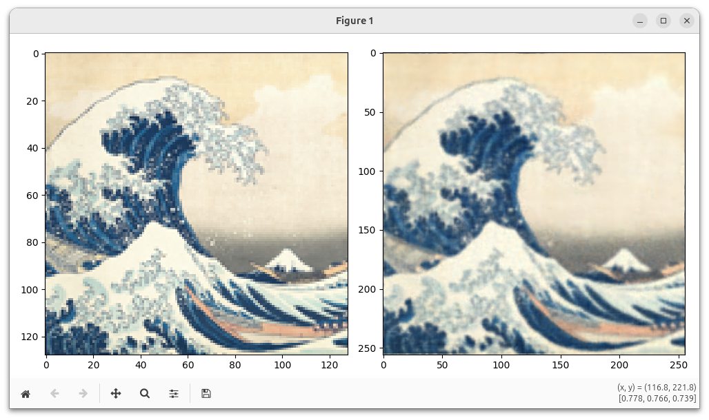
https://d38rqfq1h7iukm.cloudfront.net/media/uploads/wjakob/2024/06/coopvec-screenshot.png

The optimization uses the Adam optimizer (dr.opt.Adam) optimizer and a gradient scaler (dr.opt.GradScaler) for adaptive mixed-precision training.

from tqdm.auto import tqdm
import imageio.v3 as iio
import drjit as dr
import drjit.nn as nn
from drjit.opt import Adam, GradScaler
from drjit.auto.ad import Texture2f, TensorXf, TensorXf16, Float16, Float32, Array2f, Array3f

# Load a test image and construct a texture object
ref = TensorXf(iio.imread("https://d38rqfq1h7iukm.cloudfront.net/media/uploads/wjakob/2024/06/wave-128.png") / 256)
tex = Texture2f(ref)

# Establish the network structure
net = nn.Sequential(
    nn.TriEncode(16, 0.2),
    nn.Cast(Float16),
    nn.Linear(-1, -1, bias=False),
    nn.LeakyReLU(),
    nn.Linear(-1, -1, bias=False),
    nn.LeakyReLU(),
    nn.Linear(-1, -1, bias=False),
    nn.LeakyReLU(),
    nn.Linear(-1, 3, bias=False),
    nn.Exp()
)

# Instantiate a random number generator to initialize the network weights
rng = dr.rng(seed=0)

# Instantiate the network for a specific backend + input size
net = net.alloc(
    dtype=TensorXf16,
    size=2,
    rng=rng
)

# Convert to training-optimal layout
weights, net = nn.pack(net, layout='training')
print(net)

# Optimize a single-precision copy of the parameters
opt = Adam(lr=1e-3, params={'weights': Float32(weights)})

# This is an adaptive mixed-precision (AMP) optimization, where a half
# precision computation runs within a larger single-precision program.
# Gradient scaling is required to make this numerically well-behaved.
scaler = GradScaler()

res = 256

for i in tqdm(range(40000)):
    # Update network state from optimizer
    weights[:] = Float16(opt['weights'])

    # Generate jittered positions on [0, 1]^2
    t = dr.arange(Float32, res)
    p = (Array2f(dr.meshgrid(t, t)) + rng.random(Array2f, (2, res * res))) / res

    # Evaluate neural net + L2 loss
    img = Array3f(net(nn.CoopVec(p)))
    loss = dr.squared_norm(tex.eval(p) - img)

    # Mixed-precision training: take suitably scaled steps
    dr.backward(scaler.scale(loss))
    scaler.step(opt)

# Done optimizing, now let's plot the result
t = dr.linspace(Float32, 0, 1, res)
p = Array2f(dr.meshgrid(t, t))
img = Array3f(net(nn.CoopVec(p)))

# Convert 'img' with shape 3 x (N*N) into a N x N x 3 tensor
img = dr.reshape(TensorXf(img, flip_axes=True), (res, res, 3))

import matplotlib.pyplot as plt
fig, ax = plt.subplots(1, 2, figsize=(10,5))
ax[0].imshow(ref)
ax[1].imshow(dr.clip(img, 0, 1))
fig.tight_layout()
plt.show()

Hash grid encodings¶

The above example used a neural network with layer width 64, using the nn.TriEncode encoding layer to accelerate convergence. Such small networks are, however, quite limited in their ability to represent complex signals.

To help with this, Dr.Jit also provides a hash grid encoding (nn.HashGridEncoding), which was first introduced in Instant NGP. This data structure increases the model’s effective parameter count, providing additional memory to represent complex features while maintaining efficient network evaluations. The encoding conceptually represents trainable features on a multi-level grid, but physically stores them in a hash table for memory efficiency. During evaluation, a hash function maps grid coordinates to table entries, and the system interpolates features between adjacent grid vertices.

While hash grids work well for low-dimensional inputs, regular grid-based schemes suffer from exponential scaling: the number of memory lookups grows exponentially with the number of dimensions. To address this limitation, Dr.Jit also supports permutohedral encodings (nn.PermutoEncoding), introduced in the PermutoSDF paper. These encodings use triangles, tetrahedrons and their higher dimensional equivalents, requiring only a linear number of memory lookups with respect to dimension. This makes them particularly effective for high-dimensional inputs where regular grids become prohibitively expensive.

All previous uses of cooperative vectors and neural network modules in this documentation rely on the nn.pack() function to assemble coefficients into an efficient memory layout. However, hash grid weights cannot participate in this packing process since they use a different memory layout and potentially incompatible type representations. To incorporate a hash grid into a nn.Module, we must use an indirection via nn.HashEncodingLayer, which wraps the hash grid while keeping its parameters separate. These parameters must then be optimized independently, as shown in the following example that learns the same image using a hash grid encoding.

from tqdm.auto import tqdm
import imageio.v3 as iio
import drjit as dr
import drjit.nn as nn
from drjit.opt import Adam, GradScaler
from drjit.auto.ad import Texture2f, TensorXf, TensorXf16, Float16, Float32, Array2f, Array3f

# Load a test image and construct a texture object
ref = TensorXf(iio.imread("https://d38rqfq1h7iukm.cloudfront.net/media/uploads/wjakob/2024/06/wave-128.png") / 256)
tex = Texture2f(ref)

# Instantiate a random number generator to initialize the network weights
rng = dr.rng(seed=0)

# Create a two dimensional hash grid encoding, with 8 levels, 2 features per
# level and a scaling factor between levels of 1.5.
enc = nn.HashGridEncoding(
    Float16,
    2,
    n_levels=8,
    n_features_per_level=2,
    per_level_scale=1.5,
    rng=rng,
)

# Alternatively we can also use a permutohedral encoding. In contrast to a hash
# grid, it uses triangles, tetrahedrons and their higher dimensional
# equivalences as simplexes. Their vertex count scales linearly with dimension,
# allowing for higher dimensional inputs, while keeping the memory lookup
# overhead minimal.
# Uncomment the following lines to enable the permutohedral encoding.
# enc = nn.PermutoEncoding(
#     Float16,
#     2,
#     n_levels=8,
#     n_features_per_level=2,
#     per_level_scale=1.5,
# )
print(enc)


# Establish the network structure.
# In contrast to the previous example, we use a HashEncodingLayer, referencing
# the previously created hash grid. Its parameters will not be part of the
# packed weights, and have to be handled separately.
net = nn.Sequential(
    nn.HashEncodingLayer(enc),
    nn.Cast(Float16),
    nn.Linear(-1, -1, bias=False),
    nn.LeakyReLU(),
    nn.Linear(-1, -1, bias=False),
    nn.LeakyReLU(),
    nn.Linear(-1, -1, bias=False),
    nn.LeakyReLU(),
    nn.Linear(-1, 3, bias=False),
    nn.Exp()
)

# Instantiate the network for a specific backend + input size
net = net.alloc(TensorXf16, 2, rng=rng)

# Convert to training-optimal layout
weights, net = nn.pack(net, layout='training')
print(net)

# Optimize a single-precision copy of the parameters.
# In addition to the network weights, we also add the parameters of the
# encoding.
opt = Adam(
    lr=1e-3,
    params={
        "mlp.weights": Float32(weights),
        "enc.params": Float32(enc.params),
    },
)

# This is an adaptive mixed-precision (AMP) optimization, where a half
# precision computation runs within a larger single-precision program.
# Gradient scaling is required to make this numerically well-behaved.
scaler = GradScaler()

res = 256

for i in tqdm(range(40000)):
    # Update network state from optimizer
    weights[:] = Float16(opt['mlp.weights'])
    # Update the encoding parameters as well
    enc.params[:] = Float16(opt['enc.params'])

    # Generate jittered positions on [0, 1]^2
    t = dr.arange(Float32, res)
    p = (Array2f(dr.meshgrid(t, t)) + rng.random(Array2f, (2, res * res))) / res

    # Evaluate neural net + L2 loss
    img = Array3f(net(nn.CoopVec(p)))
    loss = dr.squared_norm(tex.eval(p) - img)

    # Mixed-precision training: take suitably scaled steps
    dr.backward(scaler.scale(loss))
    scaler.step(opt)

# Done optimizing, now let's plot the result
t = dr.linspace(Float32, 0, 1, res)
p = Array2f(dr.meshgrid(t, t))
img = Array3f(net(nn.CoopVec(p)))

# Convert 'img' with shape 3 x (N*N) into a N x N x 3 tensor
img = dr.reshape(TensorXf(img, flip_axes=True), (res, res, 3))

import matplotlib.pyplot as plt
fig, ax = plt.subplots(1, 2, figsize=(10,5))
ax[0].imshow(ref)
ax[1].imshow(dr.clip(img, 0, 1))
fig.tight_layout()
plt.show()